Rod Cutting (Dynamic Programming)

Problem : Assume a company buys long steel rods and cuts them into shorter rods for sale to its customers. If each cut is free and rods of different lengths can be sold for different amounts, we wish to determine how to best cut the original rods to maximize the revenue.

This problem can be solved using dynamic programming. Key steps in a dynamic programming solution are

• Characterize the optimality – formally state what properties an optimal solution exhibits
• Recursively define an optimal solution – analyze the problem in a top-down fashion to determine how subproblems relate to the original
• Solve the subproblems – start with a base case and solve the subproblems in a bottom-up manner to find the optimal value
• Reconstruct the optimal solution – (optionally) determine the solution that produces the optimal value

Thus the process involves breaking down the original problem into subproblems that also exhibit optimal behavior. While the subproblems are not usually independent, we only need to solve each subproblem once and then store the values for future computations.

Dynamic Programming Solution

Let us first formalize the problem by assuming that a piece of length i has price p_i. If the optimal solution cuts the rod into k pieces of lengths i₁, i₂, … , i_k, such that n = i₁ + i₂ + … + i_k, then the revenue (r_n) for a rod of length n is

Therefore the optimal value can be found in terms of shorter rods by observing that if we make an optimal cut of length i (and thus also giving a piece of length n-i) then both pieces must be optimal(and then these smaller pieces will subsequently be cut). Otherwise we could make a different cut which would produce a higher revenue contradicting the assumption that the first cut was optimal. Hence we can write the optimal revenue in terms of the first cut as the maximum of either the entire rod (p_n) or the revenue from the two shorter pieces after a cut, i.e.

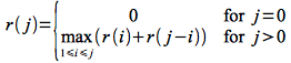
We can rewrite the optimal substructurerevenue formula recursively as

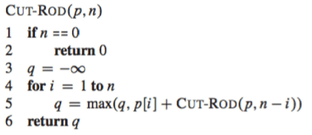
where we repeat the process for each subsequent rn-i piece. Thus we can implement this approach using a simple recursive routine

The recursion tree showing recursive calls resulting from a call CUT-ROD(p,n) for n = 4 is shown below. Each node label gives the size n of the corresponding subproblem, so that an edge from a parent with label s to a child with label t corresponding to cutting off an initial piece of size s – t and leaving a remaining subproblem of size t.

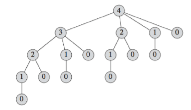If you see the recursion tree, you will see that we are actually doing a lot of extra work, because we are computing the same things over and over again. For example , in the computation for n = 4, we compute the optimal solution for n = 1 four times!.

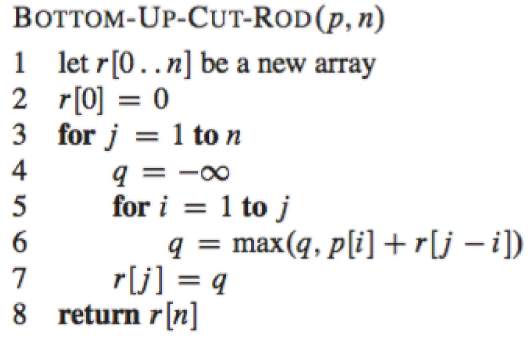
However if we can store the solutions to the smaller problems in a bottom-up manner rather than recompute them, the run time can be drastically improved (at the cost of additional memory usage). To implement this approach we simply solve the problems starting for smaller lengths and store these optimal revenues in an array (of size n+1). Then when evaluating longer lengths we simply look-up these values to determine the optimal revenue for the larger piece. We can formulate this recursively as follows

Note that to compute any r_j we only need the values r₀ to r_j-1 which we store in an array. Hence we will compute the new element using only previously computed values. The implementation of this approach is