Image Rescaling or resampling is the technique used to create a new version of an image with a different size. Increasing the size of the image is called upsampling, and reducing the size of an image is called downsampling.
Image scaling operations is not lossless. For example, if you downsample an image and then upsample the resulted image, you will get a slightly different image than the original.
Upsampling
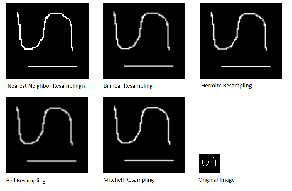
Image upsampling is illustrated with the small image below which is magnified by 400% (x4).
Downsampling
The various algorithms are applied to the binary image below which is reduced by 400% (x0.4).
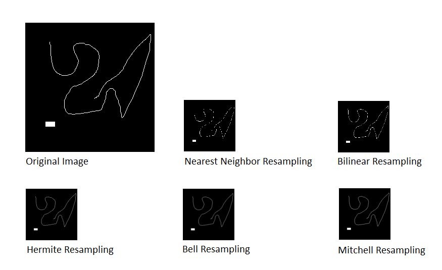
Resampling Algorithms
When an image is scaled up to a larger size, there is a question of what will be the color of the new pixels in between the original pixels. When an image is scaled down to a lower size, the question is what will be the color of the remaining pixels. There exists several answers to these questions.
Consider the case of an 1D image f(x) that we want to magnify by a factor of 2 to create the new image g(x). Mathematically, this is formulated as:
g(x) = f(x/2)
Consider a concrete example for f(x) with the sample values [2, 3, 5, 4, 3, 2, 4]. This provides the image here-after (where the image is represented by its profile, the gray levels are visualized in height). We want to double the size of the image f(x) to create the image g(x) as shown below
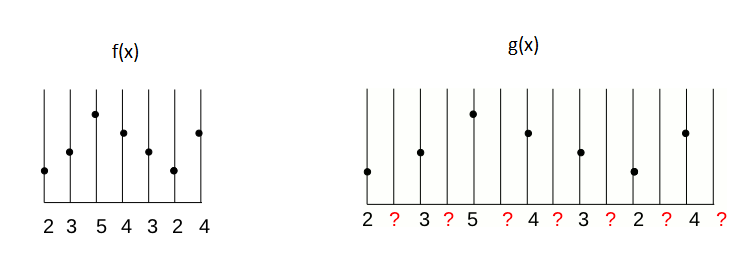
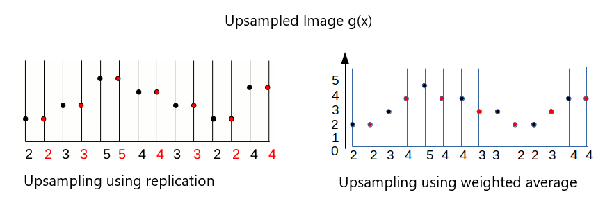
We have to determine what will be the value of the new pixels. There are two obvious answers:
- The first answer consists in doubling each original pixels. It is called Replication. To reduce the image size by a factor of n, the inverse principle of the nearest neighbor is to choose 1 pixel out of n.
- The second answer consists in using the weighted average value of the nearest known pixels according to their distance to the unknown pixel. To visualize, draw a line between two consecutive unknown pixels. Then pick the value along the line for the unknown pixels. This solution is called Linear Interpolation.
Resampling by convolution
Convolution defines a general principle for the interpolation. The interpolation kernel k(i) defines the list of neighbors to be considered and the weight assigned to them for calculating the value of the central pixel. Mathematically, this corresponds to the operation:
g(x') = \sum_{\mathclap{i}} f(x + i).k(i)By choosing the suitable filter, we can define different types of reconstruction. For example, the nearest neighbor interpolation with left priority to double the size is implemented by the convolution kernel [1, 1, 0]. Linear interpolation can be implemented by the kernel [0.5 1 0.5]. For other distances, we just use other kernels. For example, the nearest neighbor kernel for size tripling is [0, 1, 1, 1, 0] and the linear interpolation kernel is [1/3, 2/3, 1, 2/3, 1 / 3].
This implementation by convolution has several advantages:
- It provides a uniform way to implement many different types of interpolation by choosing a suitable convolution kernel.
- It is easy to extend this method to different scaling and different dimensions (2D, 3D, etc.).